Galton Board Simulator

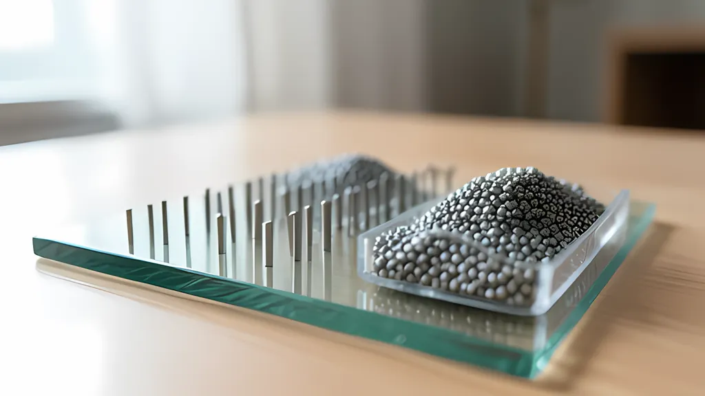
Pour lead shot through a field of pins and a hump appears. Nobody shaped it. Each pellet took its own crooked road, and the pile came out the same as last time.

That is the whole trick of the device Francis Galton called his apparatus, and the whole reason it still sits on desks. The harder questions come after the hump. Is the pile really the curve it resembles? How would you know? And when a real board disagrees with the mathematics, which one is wrong?

Galton and his frame

Galton was born on 16 February 1822 near Birmingham and died on 17 January 1911. The MacTutor biography calls him an explorer, anthropologist and statistician, a cousin of Charles Darwin, and the man who introduced regression to the mean. He was knighted in 1909.

The board was first shown, by the account Wikipedia gives, in a presentation at the Royal Institution on 27 February 1874. Galton described it in print in his 1889 book Natural Inheritance. It is a frame glazed in front, with about a quarter of an inch of depth behind the glass, a funnel at the top, rows of pins below it and a series of vertical compartments at the bottom. The pins, he wrote, are disposed “in a quincunx fashion, so that every descending shot strikes against a pin in each successive row.” Each pellet darts a step to the right or left at every pin.

His explanation is still the right one. A number of small and independent accidents befall each shot, and in most cases those that push it right roughly cancel those that push it left. So most of the shot lands near the middle, and the far compartments fill slowly. Of the law of frequency of error that the pile obeys he wrote, “It is the supreme law of Unreason.”

The same sources say what the board was for, and it was not a toy. MacTutor describes Galton as famous or infamous as the father of eugenics, and says he devoted the latter part of his life to it. The United States National Human Genome Research Institute records that he coined the word in 1883, and describes eugenics as a scientifically inaccurate theory that humans can be improved through selective breeding, linked to discrimination, racism, ableism and colonialism. Wikipedia’s account of the board adds that he meant it to illustrate reversion toward the average in heredity, an idea he made part of that program.

Counting the roads

Suppose a board has n rows and a bead goes right with chance p at every pin. A bead that goes right k times ends in bin k, counting from zero at the left, so there are n + 1 bins. The number of different roads to bin k is the binomial coefficient, the entry of Pascal’s triangle, and the chance of landing there is that coefficient times p to the power k times 1 - p to the power n - k. This is the binomial distribution. Its mean is np and its variance is np(1 - p).

Take a level board of 12 rows. There are 4,096 equally likely roads, and 924 of them end in the middle bin, so that bin should hold 22.56% of the beads. The mean is 6 and the variance is 3. Nothing about this is approximate.

The bell curve enters as a limit. Abraham de Moivre published the result in the second edition of The Doctrine of Chances in 1738: as the number of trials grows, the binomial probabilities approach the normal curve with mean np and standard deviation the square root of np(1 - p). It is a special case of the central limit theorem, which the NIST handbook summarizes by saying that a mean of many values becomes approximately normal whatever the distribution of the original variable. A bead’s bin is a sum of n small steps. That is why a board draws a bell.

The two curves are not the same thing, and a 12-row board is small enough to show the difference. The exact chance that a bead lands in bins 0 to 4 is 794 in 4,096, or 0.1938. Read straight off the normal curve at 4, with mean 6 and standard deviation 1.732, the answer is 0.1241. That is badly wrong.

The repair is old and simple. A bin is a whole number, and the curve is continuous, so bin 4 should own the stretch from 3.5 to 4.5. Asking the curve for everything up to 4.5 gives 0.1932, within 0.0006 of the truth. This half step is the continuity correction. It matters most on short boards.

The normal curve earns its place by being convenient. The handbook gives the familiar figure that 68.27% of a normal population lies within one standard deviation of the mean. On the 12-row board that band runs from about 4.3 to 7.7, and the three middle bins hold 61.2% exactly. The curve is a summary. The binomial is the law.

What a fit test says

A pile of beads never matches its law exactly, so the question is whether the mismatch is larger than chance alone would produce. The chi-square goodness-of-fit test answers that. For each bin, take the count observed minus the count expected, square it, and divide by the count expected. Add these up. If the beads really follow the stated law, the handbook says the total follows approximately a chi-square distribution whose degrees of freedom are the number of cells minus one, less one more for each parameter estimated from the data.

Here is a run anyone can repeat. Set 12 rows, a chance of 0.50 and seed 1889, pause, press Reset, then add 10,000 beads. The pile holds 10,250 beads, and the middle bin has 2,386 of them where 2,312 were expected. The outermost bin on each side is pooled with its neighbor, leaving 11 cells and 10 degrees of freedom. The statistic comes to 10.26. The handbook’s table gives 18.307 as the 5 percent critical value for 10 degrees of freedom, so the hypothesis stands, with a p-value of 0.42.

The pooling is not decoration. The chi-square approximation needs enough expected beads in every cell. The handbook gives the rule of thumb that every group should have at least five, and Wikipedia’s article on the test notes that some authors ask for five and others for ten. Outer bins that expect half a bead cannot be tested alone.

The test has plain limits. A large p-value does not prove the pile is binomial. The handbook’s own wording is that the test fails to reject. The answer also depends on how the bins are grouped, and the approximation needs a sufficient sample. And a true binomial source will still be rejected at the 5 percent level in about one run in twenty. Over 200 seeded runs of 5,000 ideal beads, the simulator rejected exactly 5 percent.

Why real boards drift

Galton claimed less than his admirers do. The outline of his columns, he wrote, approximates to the curve of frequency, and would come nearer if the rows of pins were much more numerous, the shot smaller and the compartments narrower.

Physics adds trouble of its own. A real bead does not flip a coin at each pin. It arrives with sideways speed left over from the pin before, so its steps are not independent, and it jostles its neighbors. Kozlov and Mitrofanova simulated a point ball bouncing off round nails with a coefficient of restitution. They found piles close to Gaussian for some values of that coefficient and very different from it for others. Feeding the balls evenly across the funnel mouth gave a pile far from normal.

The simulator’s physics mode shows the same thing in miniature, and reports it. On its default board at eight beads a second, the pile centers correctly but is too wide. Its variance was 1.38 times the binomial value, averaged over five seeds of 2,000 beads, and the fit test rejected every run. Dropped at two beads a second, so that beads seldom collide, the ratio fell to 1.01 and no run was rejected. Those numbers describe this model with its chosen sizes and bounce. They are not measurements of any manufactured board.

So the ideal mode and the physics mode answer different questions. The first takes each step from a published random number generator, Marsaglia’s xorshift, and is binomial by construction. The falling beads are a picture laid over that arithmetic. The second is a small mechanical model that only resembles the law.

Where the bell curve stops

The bell is a statement about sums of many independent, modest contributions. Remove any of those words and it can fail. Wikipedia’s article describes a board built by Jacobus Kapteyn whose obstacles multiply a bead’s displacement instead of adding to it. That board piles up a log-normal curve, not a normal one.

Some quantities have no bell at all. The handbook offers the Cauchy distribution as its pathological case. It looks much like a normal curve, yet its mean and standard deviation are undefined, and collecting 1,000 points estimates them no better than a single point does.

A pin board cannot tell you which kind of world you are in. It shows what follows when the conditions hold: independent steps, a fixed chance, many rows. The test beside it shows how to check a pile against that claim, and how modest the verdict has to be.